
In an Excel pivot table, you can use built-in custom calculations, for a different view of the data.
For example, in this video I set up the pivot table to show what % of monthly sales were Binders, and what % for each colour – red, blue, and black.
You can get the sample file that I used for this video on the Pivot Table Show Values As page, on my Contextures site.
Example: % of Parent Row Total
In this example, the pivot table has:
- Item and Colour in the Row area
- Month in the Column area
- Sum of Units sold, in the Values area
Follow the steps below, to show the additional sales details:
- the % for each colour’s sales – Black, Blue and Red
- compared to the item’s total sales
- in each month – Jan and Feb

Show % of Item Sales
In the pivot table screen shot below, I’ve added another copy of the Units field to the values area.
For the new field, I followed the steps below, to change the calculation settings
- Right-click one of the Units value cells
- In the pop-up menu, click Show Values As
- In the next pop-up menu, click % of Parent Row Total
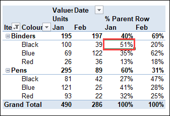
In the pivot table, the second Units field changed, to show:
- the % for each colour’s sales
- compared to the item’s total
- in each month.
For example,
- 195 Binders were sold in January
- 51% (100 units) of those January Binders were Black colour

More Pivot Table Info
For more Pivot Table tips, videos and examples, visit the following links:
Show Percent of Subtotal in Pivot Table
Pivot Table Show Values As % of Parent Total
Show Percent Of Subtotal In Pivot Table
______________________