Sort Multiple Columns in Excel Step-by-Step

ByDebra Dalgleish February 13, 2025February 11, 2025

Sorting data in Excel is quick and easy, if you only need to sort by a single column, or even two columns. For a large table, sorting can be more complicated, if you need to sort by 3 or more columns. Today, I’ll show you how to sort multiple columns in Excel so your data is quickly organized the way you need it. Whether you’re sorting by two, three, or more columns, this guide will help you through it!

Video: Sort Multiple Columns in Excel

In this short video, I show how to sort an Excel list by multiple columns. First, there’s a 2-level sort, using the Quick Sort buttons. Next, I show a 3-level sort, using the Sort dialog box.

There are written steps below the video.

Step 1: Start with Your Data

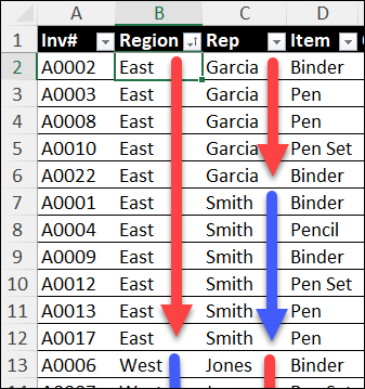
First, you need to have your data ready. For example, you might have a table with sales orders sorted by their invoice number.

Tip: Before you start sorting, make a backup copy of your Excel file. This is good practice, in case something goes wrong while sorting.

But now, you need to do a report, and you want to sort it by region and then by the sales rep within each region.

Here’s what your data might look like:

Step 2: Using Quick Sort for Simple Sorting

If you only have a couple of columns to sort, the quickest way is to use the Quick Sort buttons. You can find these buttons on your Quick Access Toolbar or the Data tab in Excel. Here’s how:

Select any cell in the column you want to sort.
Click the A to Z button to sort alphabetically.
Next, sort the other column. For example, if you want to sort by region, select the region column and click Z to A.

Now your list should show the regions in alphabetical order, with the sales reps sorted within each region.

Step 3: Plan Your Sort Steps

When sorting, remember to start with the least important column first.

For this example, we want this sorting structure:

Regions A-Z
Sales reps A-Z, under each region.

Sales reps are level 2 in the sorted results that we want, so they’ll be sorted first. Regions will be sorted second

Step 4: Use Sort Dialog Box for More Levels

If you want to do a more complex sort, like sorting by three levels (for example, sales rep, item sold, and cost), you should use the Sort dialog box:

Select any cell in your table.
Go to the Data tab and click on Sort.

This will open the Sort window. Here you can set multiple levels of sorting:

In the first dropdown, select the column you want to sort by first (in this example, it’s the sales rep).
Then click Add Level to add more sorting criteria (like items sold and cost).
Make sure to set the order for each column (A to Z for names, smallest to largest for costs).

Click OK to see your sorted data.

Step 5: Review the Sorted Data

After sorting, take quick look at your sorted data. Make sure that everything looks right and that the rows of data didn’t get jumbled accidentally.

That “jumbling” can happen if the entire table didn’t get sorted, just some of the columns. Usually, that’s caused by a blank column somewhere in the list.

If something seems off, you can always hit Undo to go back to the original order.

More Sorting Tips

For more Excel multi-column sorting tips, and to get the sample file, go to the Sort Multiple Columns in Excel page, on my Contextures site.

Also, get tips for safely sorting Excel data, to avoid problems. For example, see how you can avoid a VLOOKUP sorting problem that I ran into!